Use a portable voltage source 12 - 400V DC, powered by a car battery. Measure current I and voltage ΔV using a portable or embedded processor and record measurements at 900 samples/second.
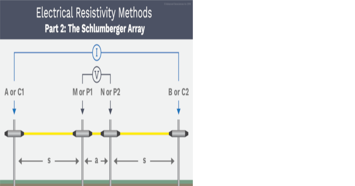
1. Apply Current I into the ground through 2 electrodes (A and B) equidistant from the measuring point (MP).
2. Measure voltage response using 2 electrodes (M and N) closely spaced around MP.
3. Record natural voltage (SP) before applying power to M and N.
4. Start recording voltage measurements using embedded processor such as Raspberry Pi.
5. Apply power to M and N for 3 seconds. Cut off power for 1 second. Apply power to M and N for 3 seconds. Cut off power. Utilisez une source de tension portable de 12 à 400 V CC, alimentée par une batterie de voiture. Mesurez le courant I et la tension ΔV à l'aide d'un processeur portable ou intégré et enregistrez les mesures à 900 échantillons/seconde.
=============================================================================================
1. Appliquez le courant I dans le sol à travers 2 électrodes (A et B) équidistantes du point de mesure (MP).
v2. Mesurez la réponse en tension à l'aide de 2 électrodes (M et N) étroitement espacées autour de MP.
3. Enregistrez la tension naturelle (SP) avant d'appliquer l'alimentation à M et N.
4. Commencez à enregistrer les mesures de tension à l'aide d'un processeur intégré tel que Raspberry Pi.
5. Appliquez l'alimentation à M et N pendant 3 secondes. Coupez l'alimentation pendant 1 seconde. Appliquez l'alimentation à M et N pendant 3 secondes. Coupez l'alimentation.
============================================================================================= ============================================================================================= How to use the program's output.=============================================================================================
Comment utiliser l'information sortie du programme.============================================================================================= ============================================================================================= Referrring to the graphical display of data at right: 6. Review graphical display to find SP and voltage response. V - SP = ΔV.
7. Record MN/2, AB/2, I, ΔV and SP in data table.
8. Use AB/2, MN/2 to calculate geometric factor G.
9. Calculate apparent resistivity ρ = G * ΔV/I.
10. Record ρ in data table with MN/2, AB/2, I, ΔV and SP.
At this location, it appears that SP = 0.01mV and V = 1,450mV: So ΔV = 1,449mV
============================================================================================= 6. Examinez l'affichage graphique pour trouver la réponse SP et la tension. V - SP = ΔV.
7. Enregistrez MN/2, AB/2, I, ΔV et SP dans le tableau de données.
8. Utilisez AB/2, MN/2 pour calculer le facteur géométrique G.
9. Calculez la résistivité apparente ρ = G * ΔV/I.
10. Enregistrez ρ dans le tableau de données avec MN/2, AB/2, I, ΔV et SP.
À cet endroit, il apparaît que SP = 0,01 mV et V = 1 450 mV : Donc ΔV = 1 449 mV